Bayesian Data Analysis

Single Parameter Normal

Prof. Niamh Cahill (she/her)

Estimating \(\mu\) from a Normal Distribution

To do Bayesian inference:

• Start off with prior probability distribution to quantify information related to \(\mu\) - example in blue with \(\mu \sim N(4,0.5^2)\)

• Collect data, \(y\), assume y has a mean \(\bar{y} = 0\) and that n = 10.

• Define the relationship between \(y\) and \(\mu\) through the likelihood function - example in red with \(y_i \sim N(\mu, \sigma = 1)\).

  • we’re assuming \(\sigma\) is known here.

• Use Bayes’ rule to update the prior into the posterior distribution \(p(\mu|y) \sim N(?,?)\).

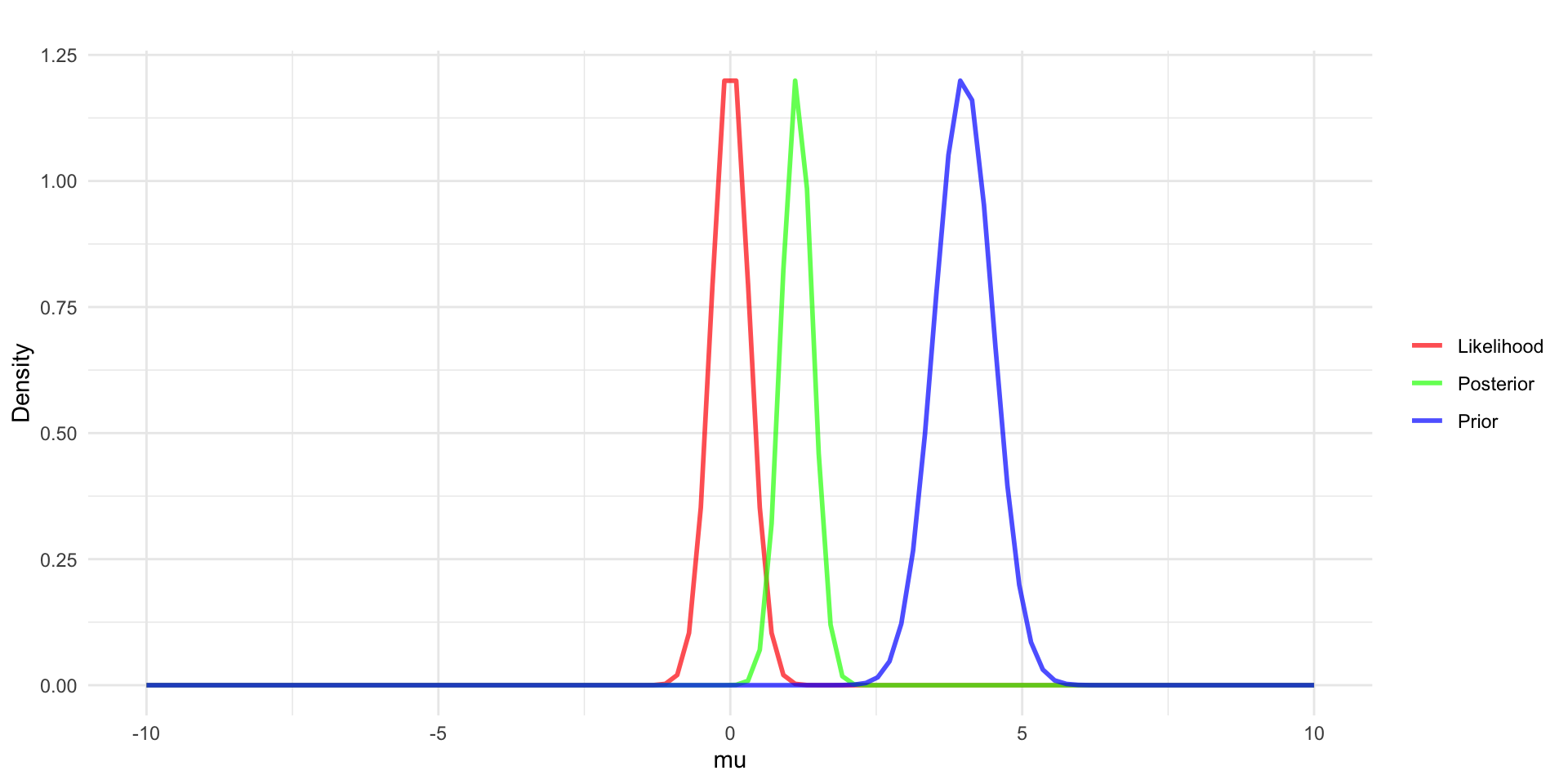
Estimating \(\mu\) from a Normal Distribution

To do Bayesian inference:

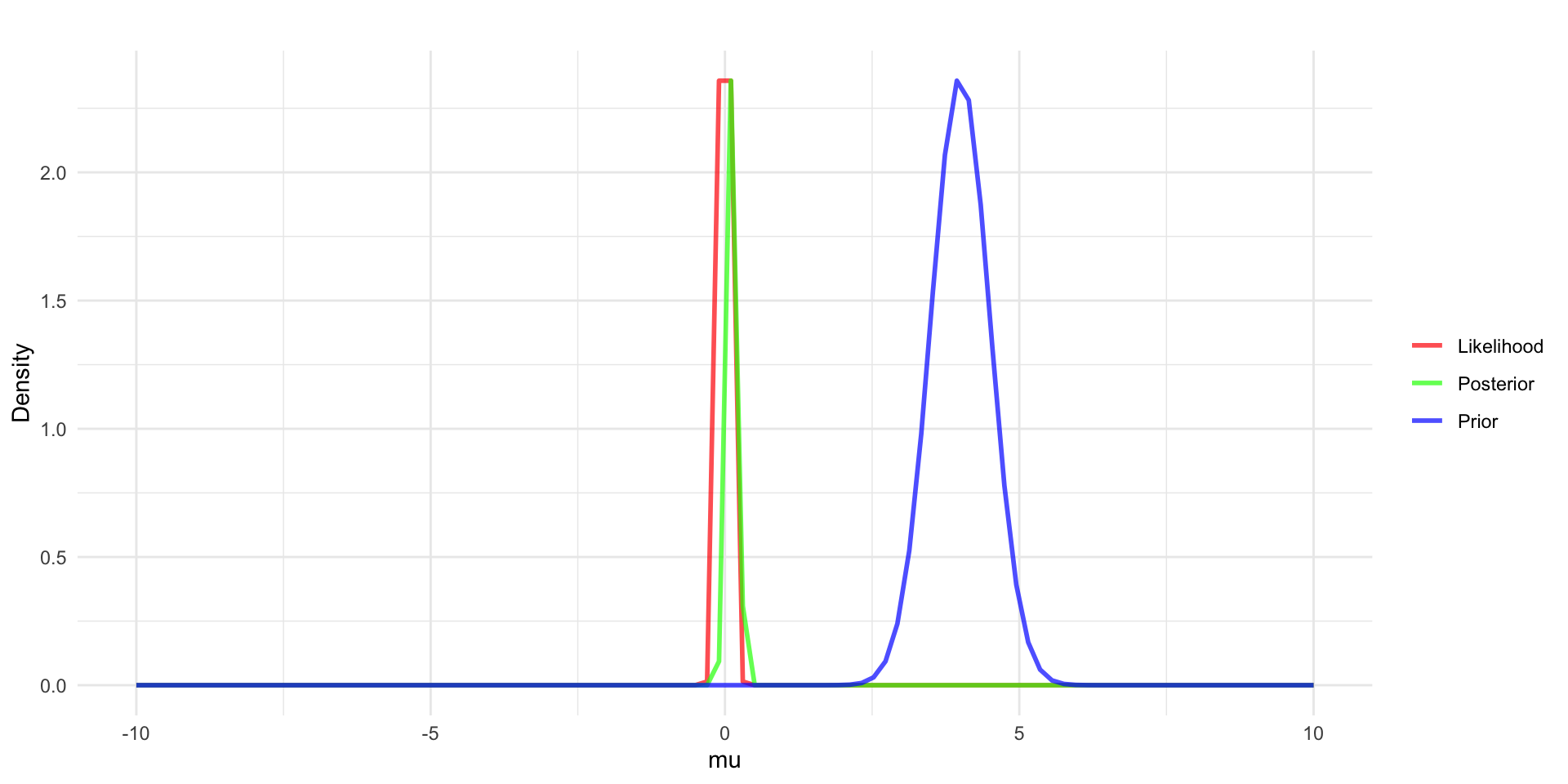
• Start off with prior probability distribution to quantify information related to \(\mu\) - example in blue with \(\mu \sim N(4,0.5^2)\)

• Collect data, \(y\), assume y has a mean \(\bar{y} = 0\) and that n = 10.
  

• Define the relationship between \(y\) and \(\mu\) through the likelihood function - example in red with \(y_i \sim N(\mu, \sigma = 2)\).

  • we’re assuming \(\sigma\) is known here.

• Use Bayes’ rule to update the prior into the posterior distribution \(p(\mu|y) \sim N(?,?)\).

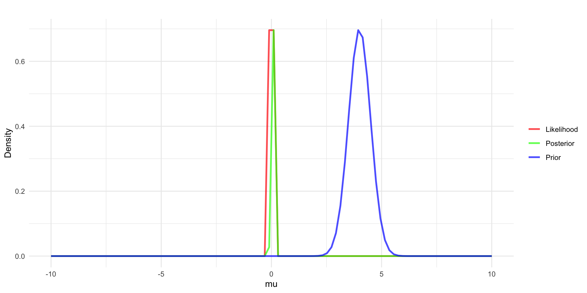
Estimating \(\mu\) from a Normal Distribution

To do Bayesian inference:

• Start off with prior probability distribution to quantify information related to \(\mu\) - example in blue with \(\mu \sim N(4,0.5^2)\)

• Collect data, \(y\), assume y has a mean \(\bar{y} = 0\) and that n = 500.

• Define the relationship between \(y\) and \(\mu\) through the likelihood function - example in red with \(y_i \sim N(\mu, \sigma = 1)\).

  • we’re assuming \(\sigma\) is known here.

• Use Bayes’ rule to update the prior into the posterior distribution \(p(\mu|y) \sim N(?,?)\).

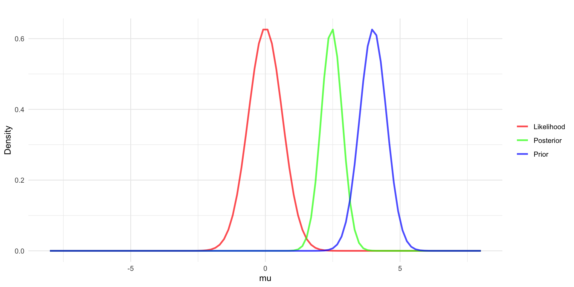
Estimating \(\mu\) from a Normal Distribution

To do Bayesian inference:

• Start off with prior probability distribution to quantify information related to \(\mu\) - example in blue with \(\mu \sim N(4,0.5^2)\)

• Collect data, \(y\), assume y has a mean \(\bar{y} = 0\) and that n = 500.

• Define the relationship between \(y\) and \(\mu\) through the likelihood function - example in red with \(y_i \sim N(\mu, \sigma = 2)\).

  • we’re assuming \(\sigma\) is known here.

• Use Bayes’ rule to update the prior into the posterior distribution \(p(\mu|y) \sim N(?,?)\).

Estimating \(\sigma \text{ } (\tau = 1/\sigma^2)\) from a Normal Distribution

To do Bayesian inference:

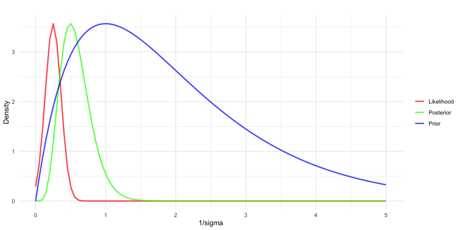
• Start off with prior probability distribution to quantify information related to \(\tau = 1/\sigma^2\) - example in blue with \(\tau = 1/\sigma^2 \sim gamma(2,1)\)

• Collect data, \(y\), assume y has a standard deviation \(s = 2, 1/s^2 = 0.5\) and that n = 10.
  

• Define the relationship between \(y\) and \(\tau\) through the likelihood function - example in red with \(y_i \sim N(\mu = 0, \sigma^2 = 1/\tau)\).

  • we’re assuming \(\mu\) is known here.

• Use Bayes’ rule to update the prior into the posterior distribution \(p(\tau|y) \sim gamma(?,?)\).

Estimating \(\sigma \text{ } (\tau = 1/\sigma^2)\) from a Normal Distribution

To do Bayesian inference:

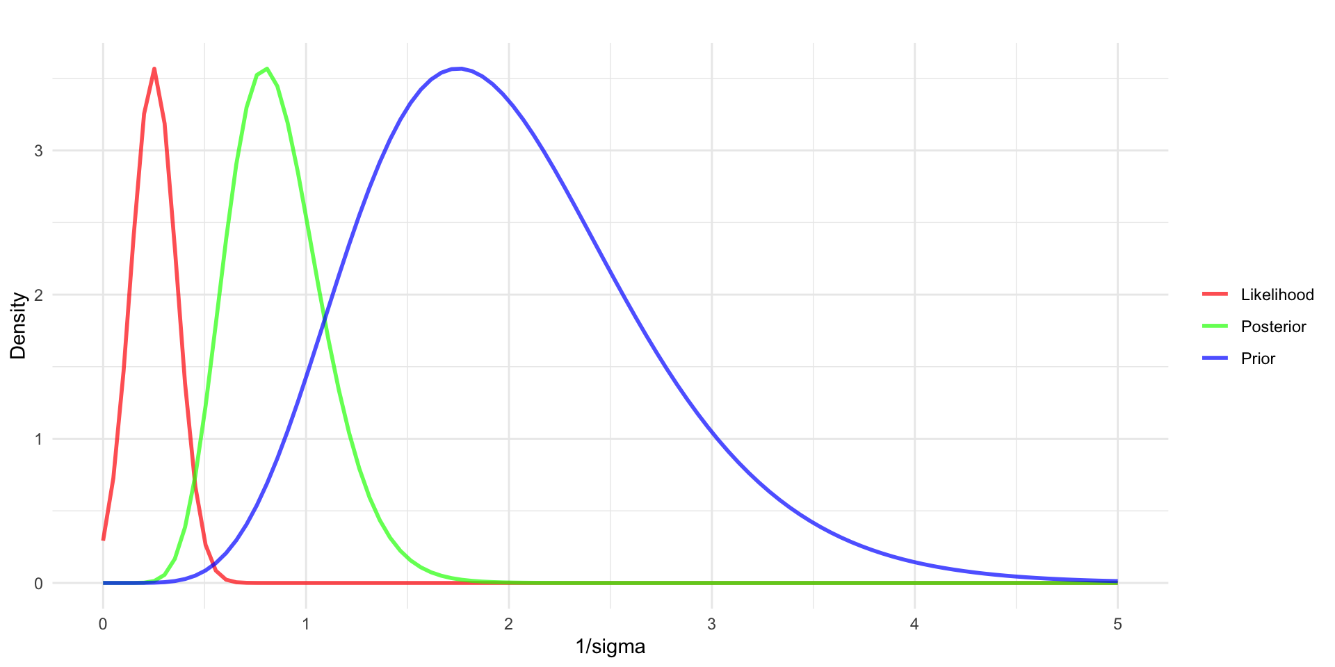
• Start off with prior probability distribution to quantify information related to \(\tau = 1/\sigma^2\) - example in blue with \(\tau = 1/\sigma^2 \sim gamma(8,4)\)

• Collect data, \(y\), assume y has a standard deviation \(s = 2, 1/s^2 = 0.5\) and that n = 10.
  

• Define the relationship between \(y\) and \(\tau\) through the likelihood function - example in red with \(y_i \sim N(\mu = 0, \sigma^2 = 1/\tau)\).

  • we’re assuming \(\mu\) is known here.

• Use Bayes’ rule to update the prior into the posterior distribution \(p(\tau|y) \sim gamma(?,?)\).

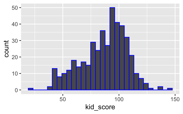
Example: Cognitive Test Scores

Data (y) are available on the cognitive test scores of three- and four-year-old children in the USA. The sample contains \(n=434\) observations.

Normal distribution with known variance

We will assume a normal model for the data where \(y_i|\mu,\sigma^2 \sim N(\mu, \sigma^2)\). Assume \(\sigma^2\) is known.

• Specify the likelihood for \(\mu\)

\(p(y|\mu, \sigma^2) = \prod_{i=1}^{n} \frac{1}{\sqrt {2\pi\sigma^2}}exp \bigg(-\frac{1}{2\sigma^2}(y_i - \mu)^2\bigg)\)

• Specify a prior for \(\mu\)

\(\mu \sim N(\mu_0, \sigma^2_{0})\)

• Use Bayes’ rule to obtain the posterior distribution

\(p(\mu|y) \propto p(y|\mu)p(\mu)\)

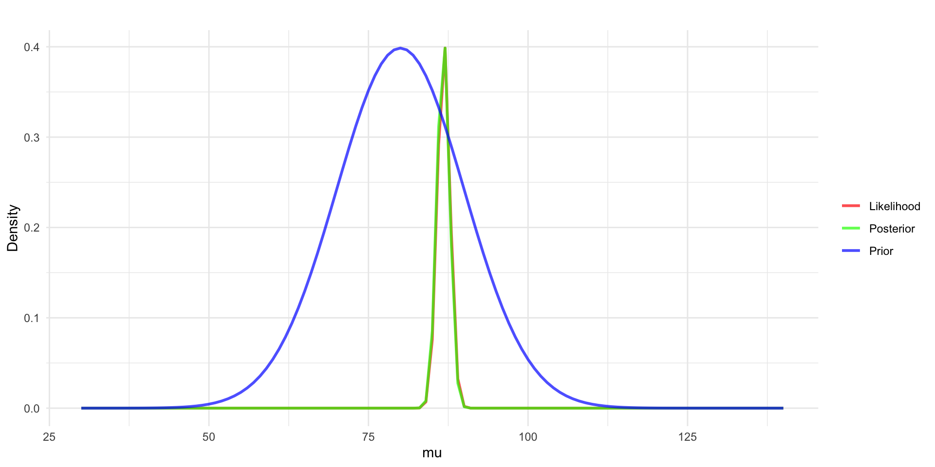
Normal distribution with known variance

• As it turns out, the posterior is also a normal distribution

\[\mu|y \sim N \bigg(\frac{n\bar{y}/\sigma^2 + \mu_0/\sigma^2_{0}}{n/\sigma^2 + 1/\sigma^2_{0}}, {\frac{1}{n/\sigma^2 + 1/\sigma^2_{0}}}\bigg)\]

• For the Kid IQ example, assuming \(\mu \sim N(\mu_0 = 80, \sigma_0 = 10)\), then \(\mu|y \sim N(86.7, 0.97)\)

Normal distribution with known mean

We will assume a normal model for the data where \(y_i|\mu,\sigma^2 \sim N(\mu, \sigma^2)\). Assume \(\mu\) is known.

• Usually work with precision i.e., \(\tau = 1/\sigma^2\)

• Specify a prior for \(\tau\)

  • Popular prior for the precision of a normal distribution is a gamma prior e.g., \(\tau \sim Gamma(a, b)\) where \(E[\tau] = \frac{a}{b}\) and \(Var[\tau] = \frac{a}{b^2}\)

  • \(p(\tau|a,b) = \frac{b^a}{\Gamma(a)}\tau^{a-1}e^{-b\tau}\) for \(\tau >0\) and \(a,b > 0\)

• Use Bayes’ rule to obtain the posterior distribution

\(p(\tau|y) \propto p(y|\tau)p(\tau)\)

Normal distribution with known mean

• As it turns out, the posterior is also a gamma distribution

\(\tau|y \sim Gamma \bigg(a + n/2, b + 1/2\sum_{i=1}^n (y_i - \mu)^2\bigg)\)

• For the Kid IQ example, assuming \(\tau \sim gamma(a = 1, b = 1)\), then \(\tau|y \sim gamma(218, 90203)\).

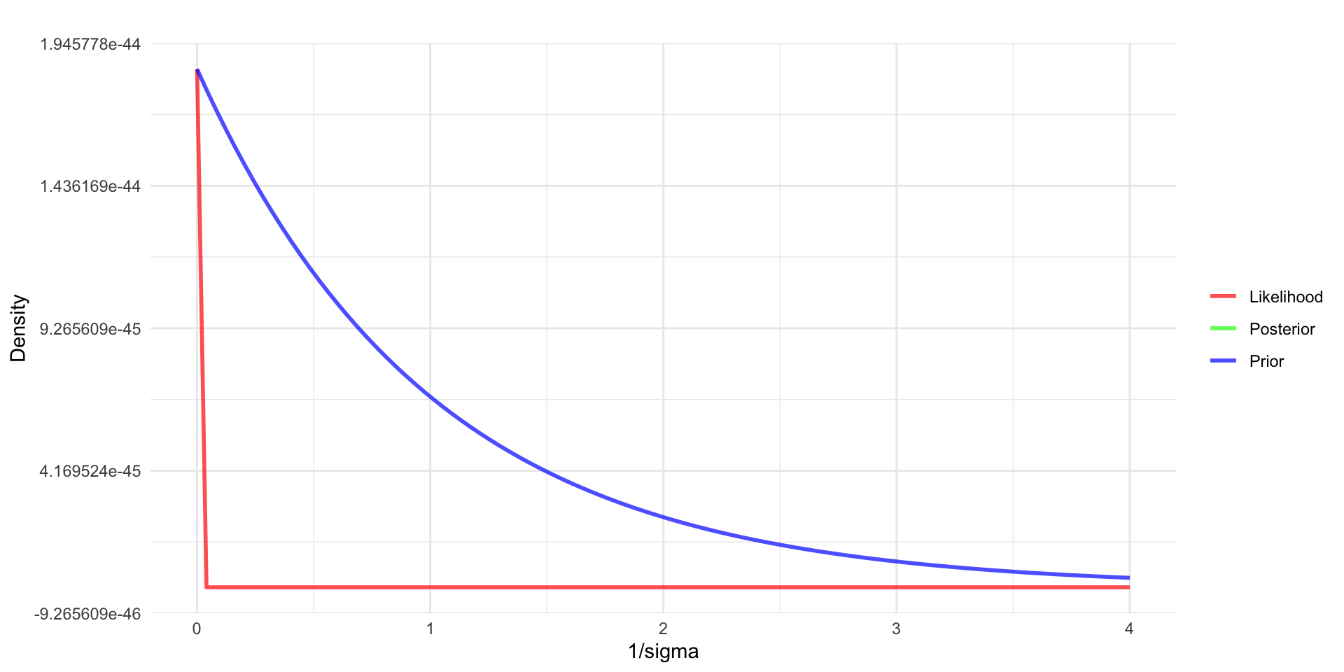
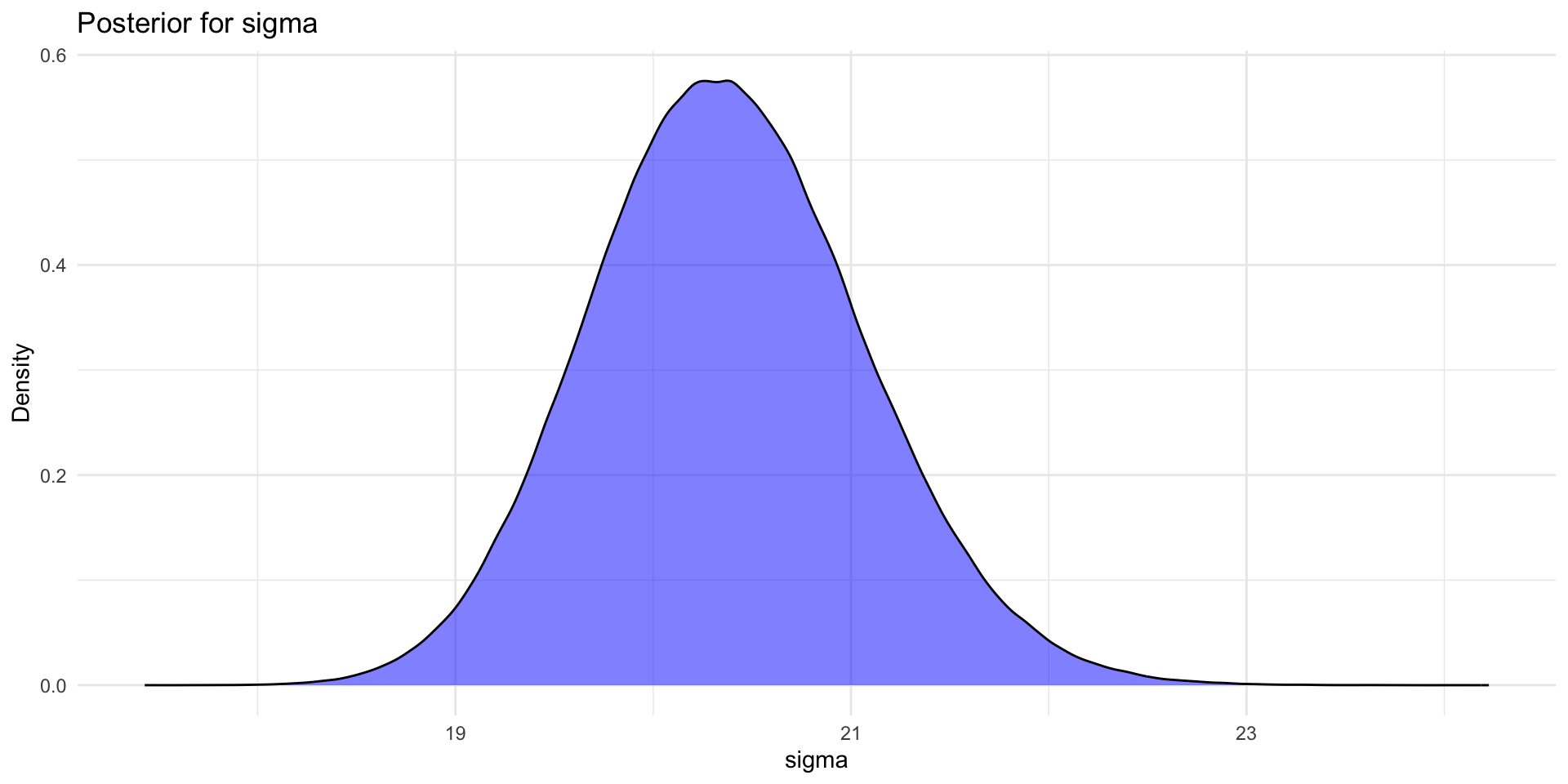
Normal distribution with known mean

• Converting back from the precision to the standard deviation, the posterior for \(\sigma\) for this example will look more like: