A Generalized Linear Model (GLM) is a flexible extension of linear regression models that allows for:
Response variables to follow a non-normal distribution, such as binomial, Poisson, or others.
Link functions to connect the linear predictor (a linear combination of independent variables) to the mean of the response variable in a way that is appropriate for its distribution.
The GLM framework consists of three components:
Random component: Specifies the probability distribution of the response variable (e.g., normal, binomial, Poisson).
Systematic component: A linear predictor formed by the independent variables and their coefficients (e.g., ( \(\eta = X\beta\) )).
Link function: Transforms the expected value of the response variable to relate it linearly to the predictors (e.g., log, logit).
Examples include logistic regression, Poisson regression, and others tailored to specific data types and distributions.
Components of a generalized linear model
Random component
\(Y\) is the response variable. \(Y \sim\) some distribution.
E.g.,
\(Y\) is continuous, \(Y \sim\) Normal.
\(Y\) is binary, \(Y \sim\) Bernoulli.
\(Y\) is # successes out of n trials, \(Y \sim\) Binomial.
\(Y\) is count, \(Y \sim\) Poisson.
Systematic component
The linear combination of explanatory variables used in the model.
You could have \(x_{2}= x_{1}^{2}\) or \(x_{3}=x_{1}x_{2}\) etc.
Link function
Let \(\mu = \mathbb{E}[Y]\). The link function, \(g\), relates \(\mu\) to the systematic component: \[g(\mu) = \eta\]
Logistic regression models: binary responses
A logistic regression model is a type of generalized linear model used for binary outcomes, where the dependent variable represents two categories (e.g., success/failure). It uses the logit link function to model the relationship between predictors and the log-odds of the outcome.
For a logistic regression model, the components are as follows:
At \(x = 0\), then \[\begin{eqnarray*}
\log\left(\frac{\pi}{1-\pi}\right) &=& \alpha \\
\frac{\pi}{1-\pi} &=& e^{\alpha}\\
\end{eqnarray*}\] So \(e^{\alpha}\) = the success odds at \(x = 0\).
Interpretation of logistic regression parameters
Interpretation of\(\beta_{1}\):
Suppose \(X\) increases from \(x\) to \(x+1\). Let \(w_1\) = the success odds at \(x\) and \(w_2\) = the success odds at \(x+1\). Then the odds change from: \[w_1 = e^{\alpha + \beta_{1}x}\] to \[\begin{eqnarray*}
w_2 &=& e^{\alpha + \beta_{1}(x+1)} \\
&=& w_{1} e^{\beta_{1}}
\end{eqnarray*}\]
i.e., increasing \(X\) by 1 unit changes the success odds by a multiplicative factor of \(e^{\beta_{1}}\)
Or, \[\frac{w_2}{w_1} = e^{\beta_{1}}\]
i.e., \(e^{\beta_{1}}\) is the odds ratio for a unit increase in \(X\).
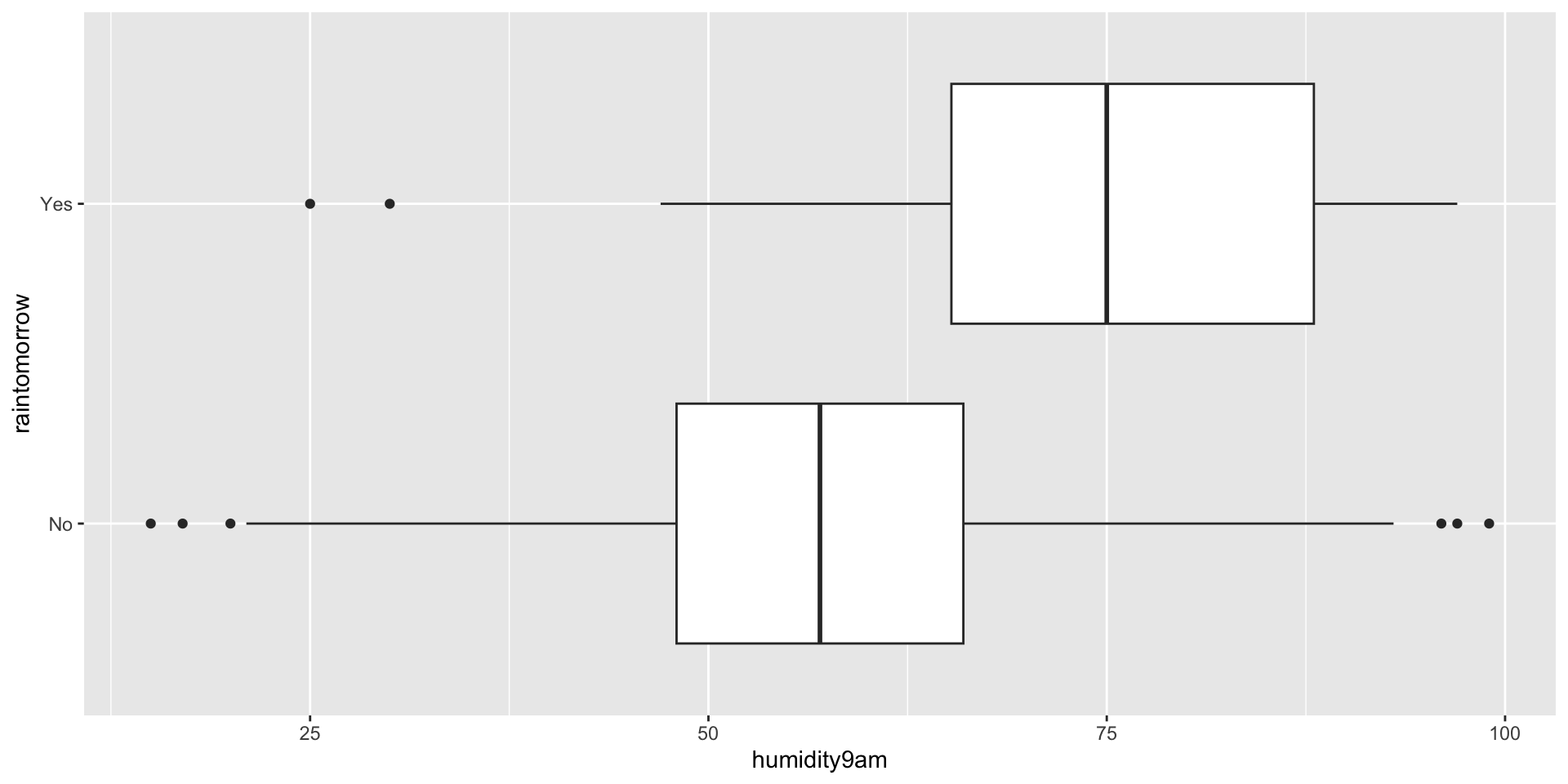
Example: Rain in Perth
Suppose we find ourselves in Australia, the city of Perth specifically. Located on the southwest coast, Perth experiences dry summers and wet winters. Our goal will be to predict whether or not it will rain tomorrow. We’re going to use today’s humidity as a predictor. Here’s a quick look at the data.
# A tibble: 280 × 3
   day_of_year raintomorrow humidity9am
         <dbl> <fct>              <int>
 1          45 No                    55
 2          11 No                    43
 3         261 Yes                   62
 4         347 No                    53
 5         357 No                    65
 6         254 No                    84
 7         364 No                    48
 8         293 No                    51
 9         304 Yes                   47
10         231 Yes                   90
# ℹ 270 more rows
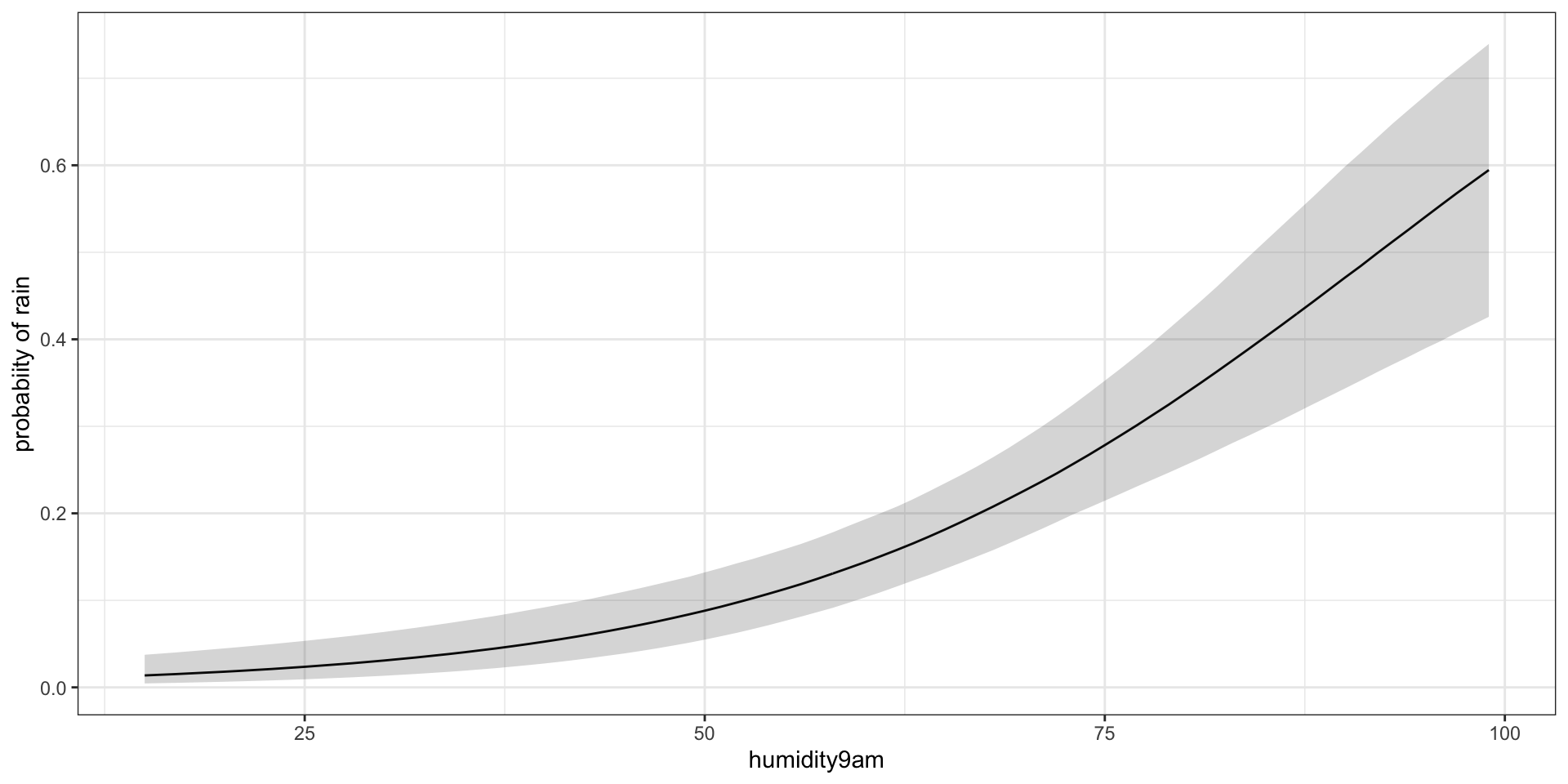
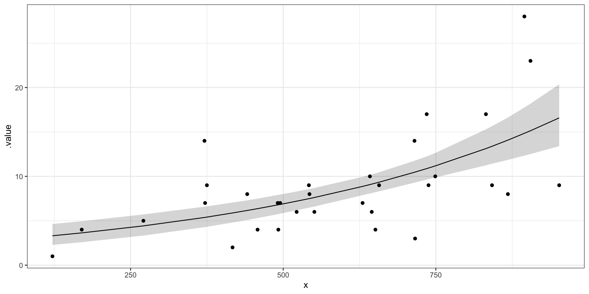
Plot the model fit for probability of rain rate by humidity
pred_summary <- m %>%gather_rvars(pi.i[pred_ind]) %>%median_qi(.value) %>%mutate(x = jags.data$x.i)ggplot(pred_summary,aes(x = x, y = .value),alpha =0.3) +geom_line() +geom_ribbon(data = pred_summary,aes(ymin = .lower, ymax = .upper), alpha =0.2) +theme_bw() +xlab("humidity9am") +ylab("probabiity of rain")
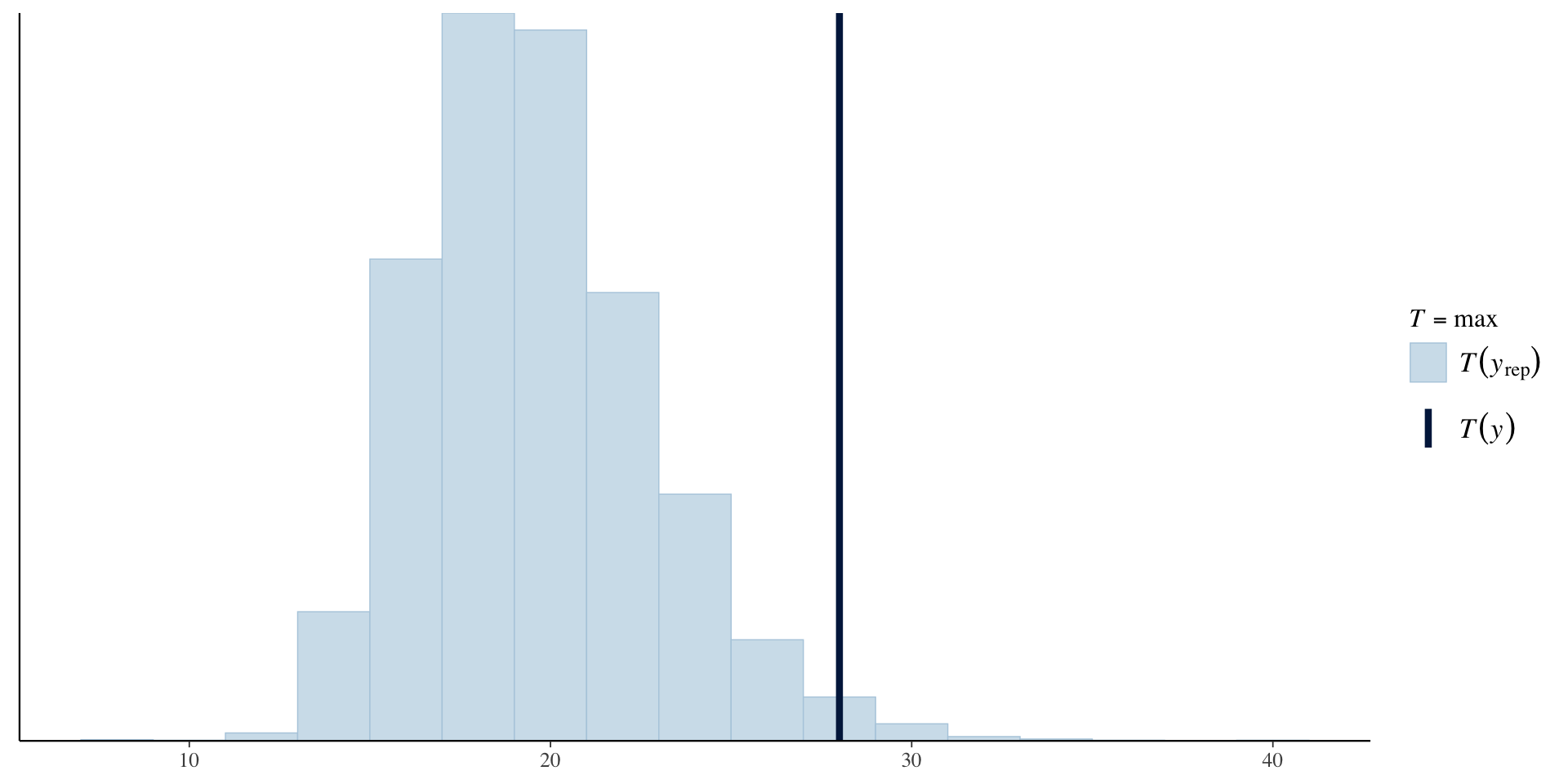
Posterior Predictive Check
Add the JAGS code for the posterior predictive check:
for(i in 1:n)
{
yrep[i] ~ dbern(pi.i[i])
}
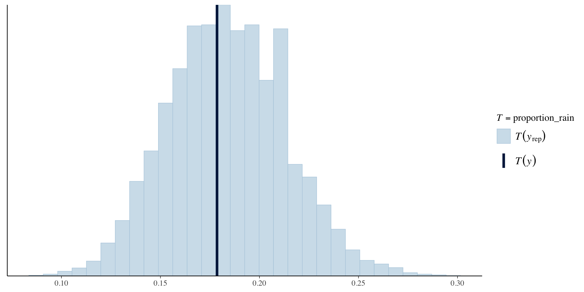
Check observed proportion of days on which it rained vs proportion of days on which it rained in each of the posterior simulated datasets.
yrep <- mod$BUGSoutput$sims.list$yrepy <- jags.data$y.iproportion_rain <-function(y){mean(y ==1)}ppc_stat(y, yrep, stat ="proportion_rain")
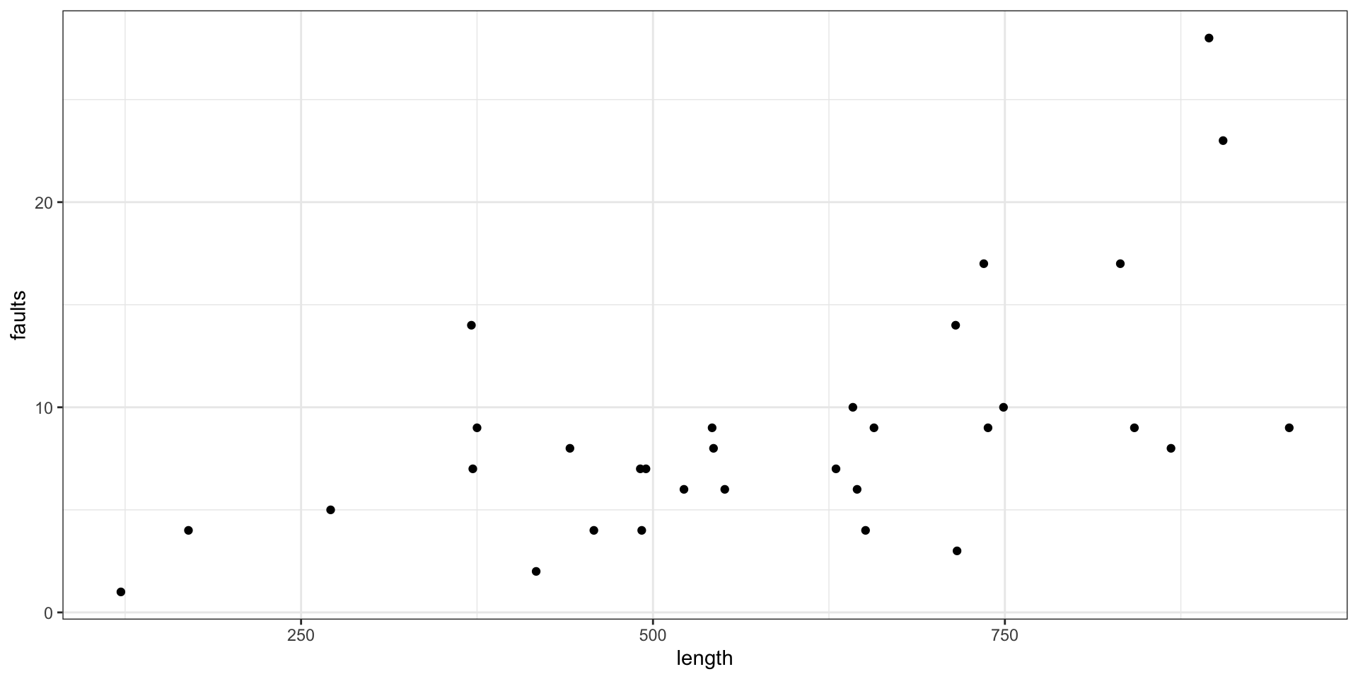
Poisson Regression
A Poisson regression model is a type of generalized linear model used for count data, where the response variable represents the number of occurrences of an event in an interval of time. It uses the log link function to relate predictors to the expected log count of the outcome.
For a Poisson regression model, the components are as follows:
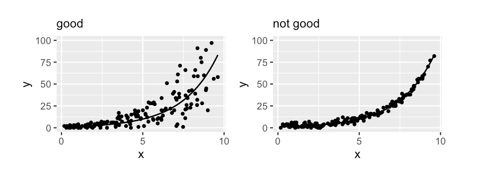
A typical value of \(y\) conditioned on \(x\) should be roughly equivalent to the variability in \(y\)
Two simulated datasets. The data on the left satisfies the Poisson regression assumption that, at any given x, the variability in y is roughly on par with the average y value. The data on the right does not, exhibiting consistently low variability in y across all x values.
Interpretation of parameter estimates
Consider the model with one predictor (\(k = 1\)):
\[log(\lambda) = \alpha + \beta x\]
Interpretation of\(\alpha\):
At \(x = 0\), then \[\begin{eqnarray*}
\log(\lambda) &=& \alpha \\
\lambda &=& e^{\alpha}\\
\end{eqnarray*}\] So \(e^{\alpha}\) = the expected count at \(x = 0\).
Interpretation of logistic regression parameters
Interpretation of\(\beta\):
Suppose \(X\) increases from \(x\) to \(x+1\). Then \(\lambda\) changes from